系列 《Transformer 原理与实现:从论文到手搓 GPT-2》 第 4 / 5 篇 进阶
系列总览 — 为什么这样组织、读它需要什么、读完能做什么 · 幻灯片 — 整个系列的精华,一份可分享的 deck
学习地图 — AI-Infra 工程师学习地图 第 4 / 14 个系列 · AI 算法工程师学习地图 第 5 / 12 个系列
- Transformer 长什么样——从一句话到下一个 token
- 一个 token 的旅程——训练侧与推理侧
- 手搓 GPT(上)——nanoGPT model.py 逐行解析
- 手搓 GPT(下)——nanoGPT train.py 与训一个会续写的模型
- Transformer 原理与实现:系列总结与通关自测
上一篇:手搓 GPT(上)——nanoGPT model.py 逐行解析下一篇:Transformer 原理与实现:系列总结与通关自测
本篇在系列中的位置。 《Transformer 原理与实现》系列的最后一篇。第 03 篇写好了模型,本篇写训练循环并在笔记本上训出会续写的模型;本系列到此回答完「GPT-2 怎么工作、怎么写」。接下来读《现代 LLM 结构:从 GPT-2 到今天的演进》,从今天的模型改了哪些结构开始。
上一篇的 model.py 定义了一个 GPT,但它的权重是随机数,输出是乱码。让它变成一个”会写东西”的模型,还差三样:数据(一段文本怎么变成模型能吃的整数数组)、训练循环(第二篇那一步”取 batch → 前向 → loss → 反向 → 更新”怎么写成能跑几十万步、能断点续训、能多卡的代码)、一次实际的训练(看着 loss 从 4.17 掉到 1.66、输出从乱码变成像莎士比亚台词的东西)。nanoGPT 的 train.py(336 行)加 prepare.py(68 行)就是这三样。
这一篇把 train.py 按块过完,然后在一台 MacBook 上用莎士比亚全集训 2000 步(7 分钟),再把层数改成 2 和 8 各训一次——这是你第一次亲手改模型结构并看到后果。训练循环里的每个机制(混合精度、梯度累积、学习率调度、DDP)本身在工具箱与 Infra PyTorch 系列里都讲过,这里只讲它们在这个脚本里的位置和为什么在那里。
本篇要回答的核心问题是:
从一个 1.1 MB 的文本文件到一个能续写它的模型,中间每一步的代码在哪、为什么那样写?把层数从 4 改到 2 或 8,loss 和速度各会怎样?1
一、总览:三个文件、一条流水线
%% 图:nanoGPT 训练的三个文件:prepare.py 把文本编码成 uint16 的 train.bin / val.bin;train.py 用 get_batch 随机切窗口、按 model.py 建模型、跑训练循环并写 ckpt.pt;sample.py 读 ckpt.pt 用 generate 续写
flowchart TB
    TXT["input.txt:莎士比亚全集 1.1 MB"] --> PREP["data/shakespeare_char/prepare.py<br/>字符 → 整数(65 个字符的词表)"]
    PREP --> BIN["train.bin / val.bin:uint16 数组,1.0M / 0.11M 个 token<br/>meta.pkl:字符表"]
    BIN --> GB["train.py · get_batch<br/>随机切 batch_size 个长 block_size 的窗口"]
    MODEL["model.py:GPTConfig / GPT(上一篇)"] --> INIT["train.py · 模型初始化<br/>scratch / resume / gpt2"]
    GB --> LOOP["train.py · 训练循环<br/>lr → 评估 → 梯度累积 × 前向 / 反向 → clip → step"]
    INIT --> LOOP
    LOOP --> CKPT["out_dir/ckpt.pt<br/>model + optimizer + iter_num + config"]
    CKPT --> SAMPLE["sample.py<br/>加载 ckpt,model.generate() 续写"]
train.py 从上到下分九块。本文的章节安排就按这九块走:
| 章 | train.py 的块 |
行号 | 内容 |
|---|---|---|---|
| 二 | (prepare.py) |
— | 字符级分词:文本 → uint16 数组 |
| 三 | 配置 | 31–75 | 72 个全局变量;configurator.py 的 exec 技巧 |
| 四 | 初始化与 I/O | 79–110 | DDP 判定、随机种子、autocast 上下文 |
| 五 | get_batch |
113–130 | 穷人的 DataLoader:随机窗口、memmap、pinned memory |
| 六 | 模型初始化 | 133–195 | 三种来源:从零、续训、GPT-2 权重;词表大小从数据来 |
| 七 | GradScaler、优化器、compile、DDP | 197–214 | 四层包装 |
| 八 | estimate_loss 与 get_lr |
216–243 | 评估;warmup + cosine |
| 九 | 训练循环 | 249–336 | 逐行:学习率、评估与 checkpoint、梯度累积、clip、step、日志 |
| 十 | 实跑 | — | 0.8M 参数、2000 步、7 分钟:loss 与样本 |
| 十一 | 改结构 | — | 2 / 4 / 8 层对比 |
| 十二 | 从 nanoGPT 到真实模型 | — | 差什么、去哪读 |
| 十三、十四 | 小结、自测 |
二、数据:prepare.py 把文本变成整数
模型吃的是 token 编号(本系列第一篇《Transformer 长什么样》第五章)。莎士比亚这个例子用字符级分词:每个不同的字符就是一个 token,词表只有 65 个(26 个字母大小写、标点、空格、换行):
# data/shakespeare_char/prepare.py(节选)
data = open('input.txt').read()                          # 1,115,394 个字符
chars = sorted(list(set(data)))                          # 65 个不同字符
stoi = { ch:i for i,ch in enumerate(chars) }             # 字符 → 编号
itos = { i:ch for i,ch in enumerate(chars) }             # 编号 → 字符
train_ids = np.array([stoi[c] for c in data[:n]], dtype=np.uint16)   # 前 90% 训练
val_ids   = np.array([stoi[c] for c in data[n:]], dtype=np.uint16)   # 后 10% 验证
train_ids.tofile('train.bin'); val_ids.tofile('val.bin')
pickle.dump({'vocab_size': 65, 'itos': itos, 'stoi': stoi}, open('meta.pkl', 'wb'))
length of dataset in characters: 1,115,394
all the unique characters:  !$&',-.3:;?ABCDEFGHIJKLMNOPQRSTUVWXYZabcdefghijklmnopqrstuvwxyz
vocab size: 65
train has 1,003,854 tokens
val has 111,540 tokens
三个决定:uint16(词表 < 65536,两字节够,文件是文本的两倍大而不是 8 倍);训练 / 验证按 9 : 1 切开(《LLM 时代的经典机器学习(01):什么是学习——划分、泛化、过拟合与偏差-方差》:验证集要没见过);meta.pkl 存字符表,训练脚本从它读词表大小、采样脚本用它把编号翻回字符。真实预训练用 BPE 分词、词表几万到十几万(预训练系列第二篇),但”文本 → 整数数组 → 随机切窗口”这条流水线完全一样——nanoGPT 的 OpenWebText 版本只是把 65 换成 50257、把 1 MB 换成 17 GB。
三、配置:72 个全局变量与一个 exec
# -----------------------------------------------------------------------------
# default config values designed to train a gpt2 (124M) on OpenWebText
# I/O
out_dir = 'out'
eval_interval = 2000
log_interval = 1
eval_iters = 200
eval_only = False # if True, script exits right after the first eval
always_save_checkpoint = True # if True, always save a checkpoint after each eval

init_from = 'scratch' # 'scratch' or 'resume' or 'gpt2*'
# data
dataset = 'openwebtext'
gradient_accumulation_steps = 5 * 8 # used to simulate larger batch sizes
batch_size = 12 # if gradient_accumulation_steps > 1, this is the micro-batch size
block_size = 1024
# model
n_layer = 12
n_head = 12
n_embd = 768
dropout = 0.0 # for pretraining 0 is good, for finetuning try 0.1+
bias = False # do we use bias inside LayerNorm and Linear layers?
# adamw optimizer

learning_rate = 6e-4 # max learning rate
max_iters = 600000 # total number of training iterations
weight_decay = 1e-1
beta1 = 0.9
beta2 = 0.95
grad_clip = 1.0 # clip gradients at this value, or disable if == 0.0
# learning rate decay settings
decay_lr = True # whether to decay the learning rate
warmup_iters = 2000 # how many steps to warm up for
lr_decay_iters = 600000 # should be ~= max_iters per Chinchilla
min_lr = 6e-5 # minimum learning rate, should be ~= learning_rate/10 per Chinchilla
# system
device = 'cuda' # examples: 'cpu', 'cuda', 'cuda:0', 'cuda:1' etc., or try 'mps' on macbooks

dtype = 'bfloat16' if torch.cuda.is_available() and torch.cuda.is_bf16_supported() else 'float16' # 'float32', 'bfloat16', or 'float16', the latter will auto implement a GradScaler
compile = True # use PyTorch 2.0 to compile the model to be faster
# -----------------------------------------------------------------------------

config_keys = [k for k,v in globals().items() if not k.startswith('_') and isinstance(v, (int, float, bool, str))]
exec(open('configurator.py').read()) # overrides from command line or config file
config = {k: globals()[k] for k in config_keys} # will be useful for logging
(为省篇幅删去了 wandb 与 DDP backend 三行。)默认值是 GPT-2 small 在 OpenWebText 上的复现配方:12 层 768 维、上下文 1024、每次迭代 5 × 8 次梯度累积 × 12 × 1024 ≈ 49 万 token(8 卡各 5 次)、60 万步、峰值学习率 6e-4、warmup 2000 步后 cosine 衰减到 6e-5、weight decay 0.1、梯度裁剪 1.0——这组数字就是预训练系列第五篇讨论的”训练配方”,六个优化器参数与 GPT-3 论文一致(\(\beta_2 = 0.95\) 而不是 Adam 默认的 0.999,《深度学习基础(06):优化器——从 SGD 到 AdamW 与学习率调度》讲为什么)。
dtype:有 CUDA 且支持 bf16 就用 bf16,否则 fp16(要配 GradScaler,第七章);CPU / MPS 上这一行会选 fp16,但第四章会看到 CPU 实际不用 autocast。
配置怎么改:configurator.py 是作者自称”糟糕主意”的 47 行——把命令行 --key=value 解析后 exec 进 globals(),覆盖上面的默认值;配置文件(config/train_shakespeare_char.py)也是一段被 exec 的 Python。好处是每个变量就是一个普通全局名,代码里不用写 config.xxx;代价是没有类型检查、IDE 不认识、exec 一般被认为不安全(Infra Python 系列讲 exec 与作用域)。工具箱第一篇用 dataclass 做配置是更常规的选择;理解 nanoGPT 时只要记住:train.py 里出现的每个小写全局变量都可以在命令行上 --name=value 改。config_keys 把所有基础类型的全局名收集起来,之后一起存进 checkpoint 和 wandb。
四、初始化与 I/O
# various inits, derived attributes, I/O setup

ddp = int(os.environ.get('RANK', -1)) != -1 # is this a ddp run?
if ddp:
    init_process_group(backend=backend)
    ddp_rank = int(os.environ['RANK'])
    ddp_local_rank = int(os.environ['LOCAL_RANK'])
    ddp_world_size = int(os.environ['WORLD_SIZE'])
    device = f'cuda:{ddp_local_rank}'
    torch.cuda.set_device(device)
    master_process = ddp_rank == 0 # this process will do logging, checkpointing etc.
    seed_offset = ddp_rank # each process gets a different seed
    # world_size number of processes will be training simultaneously, so we can scale
    # down the desired gradient accumulation iterations per process proportionally
    assert gradient_accumulation_steps % ddp_world_size == 0
    gradient_accumulation_steps //= ddp_world_size
else:
    # if not ddp, we are running on a single gpu, and one process
    master_process = True
    seed_offset = 0
    ddp_world_size = 1
tokens_per_iter = gradient_accumulation_steps * ddp_world_size * batch_size * block_size
print(f"tokens per iteration will be: {tokens_per_iter:,}")

if master_process:
    os.makedirs(out_dir, exist_ok=True)
torch.manual_seed(1337 + seed_offset)
torch.backends.cuda.matmul.allow_tf32 = True # allow tf32 on matmul
torch.backends.cudnn.allow_tf32 = True # allow tf32 on cudnn
device_type = 'cuda' if 'cuda' in device else 'cpu' # for later use in torch.autocast
# note: float16 data type will automatically use a GradScaler
ptdtype = {'float32': torch.float32, 'bfloat16': torch.bfloat16, 'float16': torch.float16}[dtype]
ctx = nullcontext() if device_type == 'cpu' else torch.amp.autocast(device_type=device_type, dtype=ptdtype)
DDP 判定:torchrun 启动时会给每个进程设 RANK / LOCAL_RANK / WORLD_SIZE 环境变量(Infra PyTorch 第九篇),有就是多卡。每个进程绑到自己的 GPU、用不同的随机种子(否则 8 张卡取到同样的 batch)、只有 rank 0 打日志存 checkpoint;梯度累积步数按卡数分摊——8 卡时每卡 5 次,合起来还是 40 个 micro-batch,保证不管几张卡,每次迭代的 token 数不变。这就是”改卡数不改配方”的实现。
随机种子 1337 固定,实验可复现(工具箱第六篇);TF32 让 A100 上 fp32 矩阵乘走 Tensor Core(第十三篇)。ctx 是之后每次前向都要包一层的 autocast 上下文:CUDA 上用低精度(工具箱第四篇的混合精度),CPU 上是 nullcontext()——什么都不做。注意 device_type 只认 cuda,MPS 也走 CPU 分支,所以本文的 MacBook 实跑其实是 fp32。
五、get_batch:穷人的 DataLoader
# poor man's data loader
data_dir = os.path.join('data', dataset)
def get_batch(split):
    # We recreate np.memmap every batch to avoid a memory leak, as per
    # https://stackoverflow.com/questions/45132940/numpy-memmap-memory-usage-want-to-iterate-once/61472122#61472122
    if split == 'train':
        data = np.memmap(os.path.join(data_dir, 'train.bin'), dtype=np.uint16, mode='r')
    else:
        data = np.memmap(os.path.join(data_dir, 'val.bin'), dtype=np.uint16, mode='r')
    ix = torch.randint(len(data) - block_size, (batch_size,))
    x = torch.stack([torch.from_numpy((data[i:i+block_size]).astype(np.int64)) for i in ix])
    y = torch.stack([torch.from_numpy((data[i+1:i+1+block_size]).astype(np.int64)) for i in ix])
    if device_type == 'cuda':
        # pin arrays x,y, which allows us to move them to GPU asynchronously (non_blocking=True)
        x, y = x.pin_memory().to(device, non_blocking=True), y.pin_memory().to(device, non_blocking=True)
    else:
        x, y = x.to(device), y.to(device)
    return x, y
工具箱第三篇用 Dataset + DataLoader,nanoGPT 用 18 行自己写。三件事:
np.memmap:把train.bin映射进内存而不是读进来——OpenWebText 的train.bin有 17 GB,读不进 RAM;memmap 让操作系统按需换页(Infra Python 系列讲内存映射)。每次调用重新 memmap 是绕一个已知的内存泄漏。- 随机窗口:从数据里随机挑
batch_size个起点,每个起点切block_size个 token 当x,右移一位再切当y——第二篇第二章的”目标 = 输入右移一位”就在这两行。torch.stack把batch_size个一维张量叠成[B, T],叠出来的是连续张量,所以上一篇forward里的targets.view(-1)才不报错。没有 epoch 的概念:每步随机采样,训练多久由max_iters决定——预训练的数据量大到看不完一遍时,这是常见做法。 - pinned memory +
non_blocking:CUDA 上先把x、y放进页锁定内存再异步搬到 GPU,让下一批数据的传输和当前批的计算重叠(Infra PyTorch 第四篇第九章)。第九章会看到它怎么被用上。
六、模型初始化:三种来源
# init these up here, can override if init_from='resume' (i.e. from a checkpoint)
iter_num = 0
best_val_loss = 1e9

# attempt to derive vocab_size from the dataset

meta_path = os.path.join(data_dir, 'meta.pkl')
meta_vocab_size = None
if os.path.exists(meta_path):
    with open(meta_path, 'rb') as f:
        meta = pickle.load(f)
    meta_vocab_size = meta['vocab_size']
    print(f"found vocab_size = {meta_vocab_size} (inside {meta_path})")

# model init
model_args = dict(n_layer=n_layer, n_head=n_head, n_embd=n_embd, block_size=block_size,
                  bias=bias, vocab_size=None, dropout=dropout) # start with model_args from command line

if init_from == 'scratch':
    # init a new model from scratch
    print("Initializing a new model from scratch")
    # determine the vocab size we'll use for from-scratch training
    if meta_vocab_size is None:
        print("defaulting to vocab_size of GPT-2 to 50304 (50257 rounded up for efficiency)")
    model_args['vocab_size'] = meta_vocab_size if meta_vocab_size is not None else 50304
    gptconf = GPTConfig(**model_args)
    model = GPT(gptconf)
elif init_from == 'resume':
    print(f"Resuming training from {out_dir}")
    # resume training from a checkpoint.
    ckpt_path = os.path.join(out_dir, 'ckpt.pt')
    checkpoint = torch.load(ckpt_path, map_location=device)
    checkpoint_model_args = checkpoint['model_args']
    # force these config attributes to be equal otherwise we can't even resume training
    # the rest of the attributes (e.g. dropout) can stay as desired from command line
    for k in ['n_layer', 'n_head', 'n_embd', 'block_size', 'bias', 'vocab_size']:
        model_args[k] = checkpoint_model_args[k]
    # create the model
    gptconf = GPTConfig(**model_args)
    model = GPT(gptconf)
    state_dict = checkpoint['model']
    # fix the keys of the state dictionary :(
    # honestly no idea how checkpoints sometimes get this prefix, have to debug more
    unwanted_prefix = '_orig_mod.'
    for k,v in list(state_dict.items()):
        if k.startswith(unwanted_prefix):
            state_dict[k[len(unwanted_prefix):]] = state_dict.pop(k)
    model.load_state_dict(state_dict)
    iter_num = checkpoint['iter_num']
    best_val_loss = checkpoint['best_val_loss']
elif init_from.startswith('gpt2'):
    print(f"Initializing from OpenAI GPT-2 weights: {init_from}")
    # initialize from OpenAI GPT-2 weights
    override_args = dict(dropout=dropout)
    model = GPT.from_pretrained(init_from, override_args)
    # read off the created config params, so we can store them into checkpoint correctly
    for k in ['n_layer', 'n_head', 'n_embd', 'block_size', 'bias', 'vocab_size']:
        model_args[k] = getattr(model.config, k)
# crop down the model block size if desired, using model surgery

if block_size < model.config.block_size:
    model.crop_block_size(block_size)
    model_args['block_size'] = block_size # so that the checkpoint will have the right value
model.to(device)
词表大小从数据来:prepare.py 写的 meta.pkl 里有 vocab_size = 65,脚本读到就用它——模型的 wte 和 lm_head 大小由数据决定,不是配置项。没有 meta.pkl(OpenWebText 用 GPT-2 的 BPE)就用上一篇讲的 50304。
三种来源对应 init_from 的三个取值、三种场景:
scratch:从零训(预训练)。resume:断点续训——从ckpt.pt里读回模型参数、iter_num、best_val_loss,结构超参强制用 checkpoint 里的(层数对不上就加载不了),第七章再读回优化器状态。那个_orig_mod.前缀是torch.compile包装模型后state_dict键名多出来的(Infra PyTorch 第七篇),存之前没剥干净这里就剥。真实的大规模训练里 checkpoint 与恢复是一门大学问(Infra 大规模训练系列第五篇),这 22 行是它的最小形态。gpt2*:从 OpenAI 权重出发微调——上一篇的from_pretrained。
crop_block_size:加载的 GPT-2 上下文是 1024,想用更短的就切位置表(上一篇第九章)。最后 model.to(device) 把参数搬到 GPU。
七、四层包装:GradScaler、优化器、compile、DDP
# initialize a GradScaler. If enabled=False scaler is a no-op

scaler = torch.cuda.amp.GradScaler(enabled=(dtype == 'float16'))

# optimizer

optimizer = model.configure_optimizers(weight_decay, learning_rate, (beta1, beta2), device_type)
if init_from == 'resume':
    optimizer.load_state_dict(checkpoint['optimizer'])
checkpoint = None # free up memory

# compile the model

if compile:
    print("compiling the model... (takes a ~minute)")
    unoptimized_model = model
    model = torch.compile(model) # requires PyTorch 2.0

# wrap model into DDP container

if ddp:
    model = DDP(model, device_ids=[ddp_local_rank])
四件事各一句,机制都在别处讲过:
GradScaler:只在 fp16 下启用。fp16 的指数位只有 5 位,小梯度会下溢成 0;scaler 先把 loss 乘一个大数再反向、更新前再除回来(工具箱第四篇第二章、第十三篇讲 bf16 为什么不需要)。enabled=False时它的每个方法都是空操作,所以后面的代码不用写两套。- 优化器:上一篇第十章的
configure_optimizers(二维参数才 decay);续训时把优化器状态(Adam 的两个动量)也读回来——不读回来,恢复后前几百步会因为动量从零重新估计而抖动。读完把checkpoint置None释放那份内存。 torch.compile:Infra PyTorch 第七篇;A100 上给 GPT-2 提速约 1.3–1.5 倍,代价是启动多花一分钟。MacBook 上关掉(--compile=False)。- DDP:多卡时把模型包进
DistributedDataParallel,反向时自动 all-reduce 梯度(Infra PyTorch 第九篇第三章);下面训练循环里有一处专门为它写的优化。
八、estimate_loss 与 get_lr
# helps estimate an arbitrarily accurate loss over either split using many batches
@torch.no_grad()
def estimate_loss():
    out = {}
    model.eval()
    for split in ['train', 'val']:
        losses = torch.zeros(eval_iters)
        for k in range(eval_iters):
            X, Y = get_batch(split)
            with ctx:
                logits, loss = model(X, Y)
            losses[k] = loss.item()
        out[split] = losses.mean()
    model.train()
    return out

# learning rate decay scheduler (cosine with warmup)

def get_lr(it):
    # 1) linear warmup for warmup_iters steps
    if it < warmup_iters:
        return learning_rate * (it + 1) / (warmup_iters + 1)
    # 2) if it > lr_decay_iters, return min learning rate
    if it > lr_decay_iters:
        return min_lr
    # 3) in between, use cosine decay down to min learning rate
    decay_ratio = (it - warmup_iters) / (lr_decay_iters - warmup_iters)
    assert 0 <= decay_ratio <= 1
    coeff = 0.5 * (1.0 + math.cos(math.pi * decay_ratio)) # coeff ranges 0..1
    return min_lr + coeff * (learning_rate - min_lr)
estimate_loss:训练日志里每步的 loss 只来自一个 batch,抖得厉害;评估时在训练集和验证集上各取 eval_iters 个 batch 求平均,得到一个稳定的数。model.eval() / model.train() 切换 dropout(第二篇第七章的表);@torch.no_grad() 不建图。train loss 与 val loss 的差就是过拟合的信号(《LLM 时代的经典机器学习(01):什么是学习——划分、泛化、过拟合与偏差-方差》)——第十章的实跑里能看到它逐渐拉开。
get_lr:工具箱第三篇画过的那条曲线——前 warmup_iters 步从 0 线性升到 learning_rate,之后 cosine 衰减到 min_lr,超过 lr_decay_iters 后保持 min_lr。注意它是一个纯函数,每步算一个数再写进 optimizer.param_groups(下一章第一行),没有用 PyTorch 的 LRScheduler——效果一样,代码更直白。
九、训练循环:逐行
# training loop

X, Y = get_batch('train') # fetch the very first batch
t0 = time.time()
local_iter_num = 0 # number of iterations in the lifetime of this process
raw_model = model.module if ddp else model # unwrap DDP container if needed
running_mfu = -1.0
while True:

    # determine and set the learning rate for this iteration
    lr = get_lr(iter_num) if decay_lr else learning_rate
    for param_group in optimizer.param_groups:
        param_group['lr'] = lr

    # evaluate the loss on train/val sets and write checkpoints
    if iter_num % eval_interval == 0 and master_process:
        losses = estimate_loss()
        print(f"step {iter_num}: train loss {losses['train']:.4f}, val loss {losses['val']:.4f}")
        if losses['val'] < best_val_loss or always_save_checkpoint:
            best_val_loss = losses['val']
            if iter_num > 0:
                checkpoint = {
                    'model': raw_model.state_dict(),
                    'optimizer': optimizer.state_dict(),
                    'model_args': model_args,
                    'iter_num': iter_num,
                    'best_val_loss': best_val_loss,
                    'config': config,
                }
                print(f"saving checkpoint to {out_dir}")
                torch.save(checkpoint, os.path.join(out_dir, 'ckpt.pt'))
    if iter_num == 0 and eval_only:
        break

    # forward backward update, with optional gradient accumulation to simulate larger batch size
    # and using the GradScaler if data type is float16
    for micro_step in range(gradient_accumulation_steps):
        if ddp:
            # in DDP training we only need to sync gradients at the last micro step.
            # the official way to do this is with model.no_sync() context manager, but
            # I really dislike that this bloats the code and forces us to repeat code
            # looking at the source of that context manager, it just toggles this variable
            model.require_backward_grad_sync = (micro_step == gradient_accumulation_steps - 1)
        with ctx:
            logits, loss = model(X, Y)
            loss = loss / gradient_accumulation_steps # scale the loss to account for gradient accumulation
        # immediately async prefetch next batch while model is doing the forward pass on the GPU
        X, Y = get_batch('train')
        # backward pass, with gradient scaling if training in fp16
        scaler.scale(loss).backward()
    # clip the gradient
    if grad_clip != 0.0:
        scaler.unscale_(optimizer)
        torch.nn.utils.clip_grad_norm_(model.parameters(), grad_clip)
    # step the optimizer and scaler if training in fp16
    scaler.step(optimizer)
    scaler.update()
    # flush the gradients as soon as we can, no need for this memory anymore
    optimizer.zero_grad(set_to_none=True)

    # timing and logging
    t1 = time.time()
    dt = t1 - t0
    t0 = t1
    if iter_num % log_interval == 0 and master_process:
        # get loss as float. note: this is a CPU-GPU sync point
        # scale up to undo the division above, approximating the true total loss (exact would have been a sum)
        lossf = loss.item() * gradient_accumulation_steps
        if local_iter_num >= 5: # let the training loop settle a bit
            mfu = raw_model.estimate_mfu(batch_size * gradient_accumulation_steps, dt)
            running_mfu = mfu if running_mfu == -1.0 else 0.9*running_mfu + 0.1*mfu
        print(f"iter {iter_num}: loss {lossf:.4f}, time {dt*1000:.2f}ms, mfu {running_mfu*100:.2f}%")
    iter_num += 1
    local_iter_num += 1

    # termination conditions
    if iter_num > max_iters:
        break

if ddp:
    destroy_process_group()
(删去了 wandb 的几行。)这就是工具箱第三篇那二十行的”生产版”。按执行顺序:
- 取第一个 batch,之后每次迭代内部预取下一个(第 5 步)。
raw_model是剥掉 DDP 包装的原始模型——estimate_mfu、state_dict都要在它上面调。 - 设学习率:每步算
get_lr(iter_num),写进每个参数组——第二篇第四章”AdamW 走一步”里的 \(\eta\) 就是它。 - 评估与 checkpoint:每
eval_interval步在 rank 0 上跑estimate_loss;验证 loss 创新低(或always_save_checkpoint)就存一份 checkpoint——模型 + 优化器状态 + 结构超参 + 步数 + 配置五样,缺一样都续不了训。第六章的resume读的就是这个字典。 - 梯度累积:想要每步 49 万 token 但显存放不下那么大的 batch,就分
gradient_accumulation_steps个 micro-batch,每个前向 + 反向但不更新,梯度在.grad里累加(第二篇第三章:.grad默认累加,正是为此),最后一起step。loss 除以累积步数让累加后的梯度等于大 batch 的平均梯度。with ctx是第四章的 autocast。 - 预取:前向刚提交给 GPU(异步,Infra PyTorch 第八篇),CPU 立刻去取下一个 batch——两件事重叠。第五章的 pinned memory 在这里派上用场。
- DDP 的小优化:默认 DDP 每次
backward都 all-reduce 梯度;累积 40 个 micro-batch 就通信 40 次,浪费。只在最后一个 micro-step 同步——官方写法是model.no_sync()上下文,作者直接改那个内部标志。 - 反向:
scaler.scale(loss)在 fp16 下放大 loss 再backward;bf16 / fp32 下 scaler 是空操作。 - 梯度裁剪:先
unscale_把梯度除回真实尺度,再把全部梯度的总范数裁到 1.0——工具箱第三篇说的”少一样迟早出事”的那一样,预训练系列第五篇讲它防的 loss spike。 - 更新:
scaler.step在 fp16 下检查有没有 inf / NaN(有就跳过这步)再调optimizer.step;scaler.update调整放大倍数。然后zero_grad(set_to_none=True)释放梯度显存。 - 日志:
loss.item()是一次 CPU–GPU 同步(Infra PyTorch 第八篇第七章),所以只每log_interval步做一次;MFU 用上一篇第十章的公式,前 5 步不算(还没稳定),之后做指数平滑。
第 4–9 步合起来是一次”参数更新”;iter_num 数的是更新次数,不是 micro-batch 数。
十、实跑:0.8M 参数、2000 步、7 分钟
MacBook(Apple 芯片,--device=mps)上跑 nanoGPT README 给的小配置:4 层 4 头 128 维、上下文 64、batch 12、2000 步:
python data/shakespeare_char/prepare.py
python train.py --dataset=shakespeare_char --out_dir=out-shakespeare-char-base --device=mps --compile=False \
  --eval_interval=250 --eval_iters=20 --log_interval=50 --block_size=64 --batch_size=12 \
  --n_layer=4 --n_head=4 --n_embd=128 --max_iters=2000 --lr_decay_iters=2000 --dropout=0.0
number of parameters: 0.80M
step 0:    train loss 4.1676, val loss 4.1649
step 250:  train loss 2.8491, val loss 2.8662
step 500:  train loss 2.3961, val loss 2.4026
step 750:  train loss 2.1386, val loss 2.1655
step 1000: train loss 1.8985, val loss 1.9509
step 1250: train loss 1.6965, val loss 1.8532
step 1500: train loss 1.5555, val loss 1.7179
step 1750: train loss 1.4989, val loss 1.6616
iter 1500: loss 1.5963, time 364.55ms, mfu 0.20%
real 7m34s
读这段日志:
- step 0 的 4.17 ≈ \(\ln 65 = 4.17\)——第二篇说的”随机初始化在词表上均匀乱猜”,65 个字符。
- 2000 步后 val loss 1.66:每个字符平均 \(e^{1.66} \approx 5.3\) 个候选里犹豫(工具箱第三篇的 PPL);从 65 到 5.3,它学到了英语拼写和莎士比亚的格式。
- train 与 val 从 step 1000 起拉开(1.90 / 1.95 → 1.50 / 1.66):1 MB 数据、0.8M 参数,开始过拟合;再训下去 val 会停在 1.6 左右而 train 继续降——《LLM 时代的经典机器学习(01):什么是学习——划分、泛化、过拟合与偏差-方差》的曲线。真实预训练数据远大于参数,几乎不会过拟合。
- MFU 0.2%:MPS 上 12 × 64 = 768 个 token 的小 batch 完全喂不饱硬件(
estimate_mfu还按 A100 的 312 TFLOPS 算分母);每步 320 ms 里绝大部分是 kernel 启动开销——Infra PyTorch 第八篇的 launch-bound。这个配置是为了几分钟看到结果,不是为了效率。
用 sample.py 读回 checkpoint 续写(贪心以外的采样,温度 0.8、top-k 200):
DUKE:
How that the thee when tyrants, do loge,
And in you to let this games, knee,
I bet some mee to state, he within's the you love to count
For yet cousin shakes a bid such of England's fie,
What I can a won the doof did so live!
单词一半是拼出来的,但格式全对:大写的角色名加冒号、换行、诗行的长度、莎士比亚的用词(thee、cousin、England)。这就是 0.8M 参数、7 分钟、字符级模型能做到的程度——它学的是”下一个字符是什么”,语法和词义要在更大的模型和更多数据上才会出现(预训练系列第三篇的 scaling law)。
十一、改结构:2 层、4 层、8 层
第一次改结构。其他全部不动,只改 --n_layer:
n_layer |
参数量 | step 1000 val loss | 最终 val loss(step 1750) | 每步耗时 |
|---|---|---|---|---|
| 2 | 0.40M | 2.108 | 1.822 | ≈ 0.5× |
| 4(基线) | 0.80M | 1.951 | 1.662 | 1×(约 350 ms) |
| 8 | 1.58M | 1.882 | 1.592 | ≈ 2× |
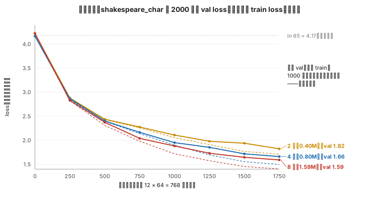
读这张表:
- 参数量:每加一层多 0.20M(一层 = attention 4 个 \(128 \times 128\) + FFN 两个 \(128 \times 512\) ≈ 0.197M),embedding 那 \(65 \times 128 + 64 \times 128\) 不随层数变——第一篇第六章的参数表在另一个模型上又对了一次。
- loss:2 → 4 层降了 0.16,4 → 8 层只降了 0.07。翻倍的参数换来的收益在递减;而且 8 层的 train / val 差距(1.41 / 1.59)比 2 层(1.71 / 1.82)大——模型越大越容易把 1 MB 的数据背下来。
- 每步耗时:层是串行的(第 \(l\) 层的输入是第 \(l-1\) 层的输出),8 层的一步大约是 4 层的两倍。同样 7 分钟,2 层能跑 4000 步、8 层只能跑 1000 步——”更深”不是免费的。
这个小实验的三个通用结论,后面每一篇都会用到:
- 参数量随层数线性增长(每层 0.20M,embedding 不变),但 loss 不是——第五篇用参数量公式解释每层多少、第六篇算每层多少 FLOPs;
- 每步耗时随层数线性增长——层是串行的,深了就慢,这是第十篇 MoE 想绕开的约束(加参数不加每 token 的计算);
- 同样的步数下更大的模型更好,但差距在缩小——”训多久、多大的模型”这个权衡就是预训练系列第三篇 scaling law 的全部内容。
十二、从 nanoGPT 到真实模型差什么
nanoGPT 是完整的:数据、模型、训练、续训、多卡、混合精度、生成都有。真实的预训练与它的差别不在”有没有”,在规模带来的新问题:
| 环节 | nanoGPT | 真实预训练(Llama 3 量级) | 去哪读 |
|---|---|---|---|
| 数据 | 1 MB 文本,prepare.py 一次编码 |
15T token,抓取 / 去重 / 过滤 / 配比是一门工程 | 预训练系列第四篇 |
| 分词 | 65 个字符 | BPE,词表 128K | 预训练系列第二篇 |
| 结构 | GPT-2:LayerNorm、位置表、GELU、MHA | RMSNorm、RoPE、SwiGLU、GQA、MoE、MTP | 本系列第五至十篇 |
| 并行 | DDP:每卡一份完整模型 | 模型放不进一张卡:张量 / 流水 / 序列 / 专家并行,ZeRO | Infra 大规模训练系列 |
| 精度 | bf16 autocast | bf16 主流,FP8 训练开始出现 | 现代 LLM 结构第十篇 |
| 稳定性 | 梯度裁剪 | loss spike 的诊断与恢复、z-loss、QK-norm | 预训练系列第五篇 |
| 容错 | resume 从单个 ckpt.pt |
万卡训练每几小时坏一张卡:分片 checkpoint、自动重启 | Infra 大规模训练系列第五、六篇 |
| 配方 | 默认值抄 GPT-3 | 用小模型消融 + scaling law 外推 | 预训练系列第三、五篇 |
| 之后 | 生成 | 后训练:SFT、RLHF / RLVR | L5 后训练系列 |
每一行 nanoGPT 都给了一个可读的最小版本;真实系统是在同一个骨架上把每一格换成能扛规模的实现。读那些系统的代码时,先在这张表里找到它对应 nanoGPT 的哪几行。
十三、本文小结
prepare.py:文本 → 字符级整数 →uint16的train.bin/val.bin(9 : 1)+meta.pkl;模型的词表大小由数据决定。train.py的配置是 72 个全局变量,默认值就是 GPT-2 small 的复现配方;configurator.py用exec让每个变量都能--name=value覆盖。get_batch用memmap+ 随机窗口 +torch.stack造[B, T]的x与右移一位的y,CUDA 上 pinned memory 异步搬运;没有 epoch。- 模型三种来源:从零(词表大小从
meta.pkl)、续训(读回参数 / 优化器 / 步数,结构超参强制一致)、GPT-2 权重;然后 GradScaler(仅 fp16)、优化器、torch.compile、DDP 四层包装。 - 训练循环每步:设学习率 → 到点评估并存 checkpoint(五样) → 梯度累积 \(k\) 个 micro-batch(loss ÷ \(k\),预取下一批,DDP 只在最后一步同步)→ unscale + 裁剪 → step / update → zero_grad → 日志与 MFU。
- 实跑:0.8M 参数、2000 步、7 分钟,val loss 4.17(\(= \ln 65\))→ 1.66,输出有莎士比亚的格式;train / val 从 1000 步起拉开——过拟合的开始。
- 改层数:参数量与每步耗时随层数线性增长,loss 收益递减——这三条是后面结构篇与 scaling law 的起点。
配套:nanogpt/(vendored 的 train.py、configurator.py、sample.py、data/shakespeare_char/prepare.py)、expected/train_shakespeare_char_{base,L2,L8}.txt、expected/sample_shakespeare_char_base.txt(ai-learning-labs/transformer-and-llm)。
十四、自测
-
默认配置下一次迭代处理多少 token?8 卡 DDP 时每卡的
gradient_accumulation_steps是多少,一次迭代的 token 数变不变?答案
\(40 \times 12 \times 1024 = 491{,}520\)。8 卡时每卡 \(40 / 8 = 5\) 次累积,总 token 数不变——脚本按卡数分摊累积步数正是为了让”配方”与卡数无关。见第四章。
-
get_batch里y为什么是data[i+1 : i+1+block_size]?用torch.stack而不是切片拼接对上一篇的forward有什么意义?答案
目标是输入右移一位(第二篇第二章)。
stack造出的是连续张量,forward里targets.view(-1)才不会因不连续报错。见第五章。 -
梯度累积时为什么要
loss = loss / gradient_accumulation_steps?如果不除会怎样?答案
.grad在 \(k\) 个 micro-batch 上累加;除以 \(k\) 后累加结果等于大 batch 的平均梯度。不除,梯度是 \(k\) 倍,等价于学习率放大 \(k\) 倍,配方就不对了。见第九章第 4 点。 -
checkpoint 里存了哪五样?少了
optimizer会怎样? -
实跑里 step 0 的 loss 为什么恰好是 4.17?如果换成 GPT-2 的 BPE 分词,这个数会是多少?
答案
\(\ln 65 = 4.17\):随机模型在 65 个字符上均匀乱猜。BPE 词表 50257 时是 \(\ln 50257 = 10.8\)。见第十章。
-
只把
n_layer从 4 改成 8,参数量、每步耗时、loss 各怎么变?为什么每步耗时随层数线性增长而不能并行?答案
参数量约翻倍(embedding 部分不变)、每步耗时约翻倍、loss 更低但收益递减。层是串行的——第 \(l\) 层的输入是第 \(l-1\) 层的输出(残差流),不能同时算;流水线并行也只是让不同 batch 的不同层同时算。见第十一章。
下一篇
到这里,一个 GPT-2 结构的模型从零到能续写走完了。但今天的 Llama、Qwen、DeepSeek 已经不是 GPT-2 的样子。下一篇《从 GPT-2 到今天的 LLM——结构演进的路线图》先把这个 GPT-2 看成一组可替换的槽位,按时间线和四条演进线排出 2019–2025 年的主要改动,再从上一篇末尾那五处改动出发——RMSNorm、RoPE、SwiGLU、GQA、去 bias——讲每一处为什么改、改了之后参数怎么数,把 config.json 里的六个数字算成 8.03B。
-
数据:
prepare.py把字符映射成 0–64 的整数存成uint16的train.bin;get_batch随机切batch_size个长block_size的窗口,目标是窗口右移一位。模型:按meta.pkl的词表大小建GPT(或从 checkpoint / GPT-2 权重恢复),包上 GradScaler、优化器、compile、DDP。循环:每步设学习率(warmup + cosine)→ 到点评估并存 checkpoint → \(k\) 个 micro-batch 各前向 + 反向累积梯度(loss ÷ \(k\),同时预取下一批)→ 裁剪 → step → zero_grad。改层数:参数量和每步耗时随层数线性增长(层是串行的),loss 的收益递减。详见第五、九、十一章。 ↩
系列 《Transformer 原理与实现:从论文到手搓 GPT-2》 第 4 / 5 篇 进阶
系列总览 — 为什么这样组织、读它需要什么、读完能做什么 · 幻灯片 — 整个系列的精华,一份可分享的 deck
学习地图 — AI-Infra 工程师学习地图 第 4 / 14 个系列 · AI 算法工程师学习地图 第 5 / 12 个系列
- Transformer 长什么样——从一句话到下一个 token
- 一个 token 的旅程——训练侧与推理侧
- 手搓 GPT(上)——nanoGPT model.py 逐行解析
- 手搓 GPT(下)——nanoGPT train.py 与训一个会续写的模型
- Transformer 原理与实现:系列总结与通关自测
上一篇:手搓 GPT(上)——nanoGPT model.py 逐行解析下一篇:Transformer 原理与实现:系列总结与通关自测
本文由 arganzheng 创作,采用 CC BY 4.0 许可协议。在保留原文作者、署名以及完整原文链接(https://arganzheng.life/nanogpt-train-py-and-training-a-model-that-writes.html)的前提下,欢迎各种形式的转载、翻译或商业引用。
COMMENTS
评论存放在 GitHub Discussions, 用 GitHub 账号登录即可发表,支持 Markdown。 想针对正文某句话说?选中那段文字,点浮出的「评论」即可划线评论;觉得哪里写错了,发表时勾上「同时提交 Issue」。 有人回复你时 GitHub 会按你的通知设置发邮件,不用守在这里。